3D Workspace
Home
Assets
Affiliate Program
Creator Program
Sign up/Log in
View Plans
DCC Bridge
martinezreyeseduardo76
10-26 23:21
Model Name
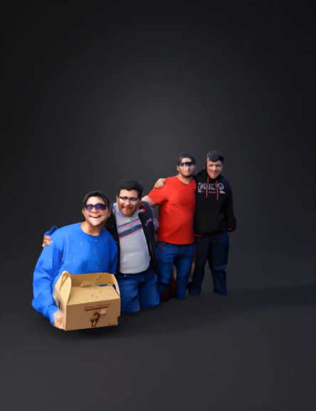
group of people 3d model
Tags
character
character realistic
character rendering
character rendering realistic
group of people
image
jpg
photorealistic
pixel
realistic
rendering
rendering realistic
representation
Input
Prompt
3D Reconstruction and Modeling Protocol for Monocular Image Input Target System: Advanced Generative AI (e.g., NeRF-based Architecture, Diffusion Model with 3D Latent Space, or High-Fidelity Photogrammetry Simulation Engine). Input Datum: Single RGB Image File: 9.jpg (Resolution: 4032×3024 pixels, Format: JPEG). Objective: To synthesize a photorealistic, textured, and geometrically accurate 3D model representation of the scene depicted in the input image 9.jpg. The output must be a fully navigable 3D asset (e.g., GLB, USDZ, or OBJ with associated texture maps and MTL file). I. Preprocessing and Data Initialization 1. Input Data Validation and Sanitization Pixel-Level Integrity Check: Execute a cyclic redundancy check (CRC) on the raw pixel data to ensure bit-level fidelity. Verify the γ correction curve is standard sRGB or approximate it via histogram analysis if EXIF data is missing. Metadata Extraction: Parse the EXIF block to retrieve key parameters: Focal Length (f), Sensor Size (s), and Image Dimensions (W×H). If f and s are unavailable, default to an f/s ratio equivalent to a 35mm full-frame effective focal length of 28mm (wide-angle estimation). Intrinsic Matrix Initialization (K): Compute the camera intrinsic matrix: K= f x 0 0 0 f y 0 c x c y 1 where f x =f y are the focal lengths in pixel units, and (c x ,c y ) is the principal point (assumed to be the image center for a rectified input). This K matrix will be the foundational parameter for the ensuing geometric transformation pipeline. 2. Initial Feature Descriptors Generation Keypoint Detection: Implement a Scale-Invariant Feature Transform (SIFT) or Accelerated-KAZE (AKAZE) algorithm to densely sample salient visual features across the image plane. Descriptor Vectorization: Generate high-dimensional feature descriptor vectors for each detected keypoint. These will serve as inputs to the downstream semantic segmentation and depth estimation modules. Semantic Segmentation (Instance-Level): Employ a trained Mask R-CNN or U-Net architecture to generate high-precision segmentation masks for all discernible object classes: Human Subjects: (4 Instances: Leftmost, Second-from-left, Third-from-left, Rightmost) Foreground Object: (Cardboard box) Background Structures: (Metal Fence/Gate, Building Facade, Sidewalk, Pavement) Sky/Foliage: (Outdoor Environment Elements) The generated masks are critical for applying differential weighting during depth inference, prioritizing the accuracy of near-field human subjects. II. Monocular Depth and Volumetric Reconstruction 3. High-Fidelity Monocular Depth Estimation (D) Depth Map Generation: Utilize a MiDaS (Monocular Depth Estimation) or equivalent state-of-the-art Convolutional Neural Network (CNN) architecture (e.g., Vision Transformer-based model) pre-trained on large-scale datasets (e.g., NYU Depth V2, KITTI) to predict a high-resolution, pixel-wise relative depth map D(u,v) from the input RGB image I(u,v). Relative to Metric Scale Conversion: The estimated depth map D is inherently relative (up to a scale and shift). Apply an Anchor Object Scaling Heuristic: Identify a subject (e.g., the rightmost human, estimated average male height H avg ≈1.75m) within a tight bounding box B ref . Use the projected size of this reference subject in the image plane and its corresponding relative depth D ref to derive a global scale factor S. Convert the relative depth map to an approximate metric depth map: D metric =S⋅D+T, where T is a minimal translational offset (assumed 0 for simplicity). This is the most crucial step for achieving a geometrically plausible 3D scene. 4. Point Cloud Generation and Filtering Back-Projection: Project each pixel (u,v) with its corresponding metric depth D metric (u,v) back into 3D space using the calibrated intrinsic matrix K and the standard pinhole camera model equation: P 3D =D metric (u,v)⋅K −1 ⋅p 2D where p 2D =[u,v,1] T . This yields an initial, unorganized 3D point cloud P. Outlier Removal: Apply a Statistical Outlier Removal (SOR) filter to eliminate spurious points resulting from depth discontinuities or estimation noise. Specifically, filter points whose mean distance to their k-nearest neighbors (k=10) exceeds 1.5 standard deviations of the global mean distance. 5. Volumetric Scene Representation (NeRF Synthesis) NeRF Initialization: Instantiate a Neural Radiance Field (NeRF) architecture. The network should map 5D coordinates (position x,y,z and view direction θ,ϕ) to a volume density (σ) and an emitted RGB color (c). Training with Pseudo-Ground Truth: Train the NeRF model using the input image I as the primary 2D supervisory signal and the generated 3D point cloud P (or a derived set of depth-constrained 3D rays) as the pseudo-ground truth for volumetric distribution. Positional Encoding: Apply high-frequency positional encoding to the input 3D coordinates to facilitate the representation of fine geometric detail (e.g., the patterns on the fence, the texture of the cardboard box). Use L=10 frequency bands for maximum fidelity. Optimization: Optimize the NeRF's multilayer perceptron (MLP) weights via a stochastic gradient descent variant (e.g., AdamW) minimizing the ray-color reconstruction loss (Mean Squared Error) and incorporating a total variation loss on the σ values to promote smooth density fields. III. Mesh Generation and Final Asset Export 6. Mesh Extraction (Marching Cubes Algorithm) Density Thresholding: Define a density threshold σ thresh within the trained NeRF's volumetric space that delineates the boundary between occupied and empty space. Mesh Generation: Apply the Marching Cubes algorithm to the sampled density grid (e.g., 512 3 resolution) derived from the NeRF's predicted σ values. This process will extract an explicit surface mesh M (a collection of vertices and triangular faces) that approximates the geometry of the scene. Remeshing and Simplification: Apply a Quadric Error Metric (QEM)-based mesh decimation algorithm to reduce the polygon count while preserving critical features, especially around the human subjects and sharp architectural edges. 7. Texture Projection and UV Mapping UV Atlas Generation: Generate a non-overlapping UV coordinate system for the mesh M using an Atlas Packing algorithm. Texture Projection: Project the original input image I onto the generated mesh M using the camera parameters K and the identity extrinsic matrix E (since the coordinate system is camera-centric). This RGB projection constitutes the base texture map T base . Inpainting and Seam Remediation: Use a Generative Adversarial Network (GAN) or a Diffusion Inpainting model to synthesize occluded back-faces and fill in texture seams and artifacts resulting from the single-view projection. The inpainting must be contextually coherent (e.g., extrapolate the back of the human subjects' heads and the obscured sections of the building). 8. Final Asset Compilation and Export Normals Calculation: Compute per-vertex and per-face normals for shading consistency. Material Definition: Define a standard PBR (Physically Based Rendering) material set, utilizing the base texture T base for the Albedo channel. Estimate roughness and metallic maps heuristically based on semantic segmentation (e.g., metal fence → low roughness, high metallic; clothing → high roughness, zero metallic). Output File Format: Export the complete 3D scene graph as a GLTF/GLB asset (Geometry M, UV maps, PBR textures, and calibrated 3D camera pose), ensuring compliance with Khronos Group specifications for maximum interoperability.
Detailed Info
Related Models
Enter invite code
Enter invite code to get credits!