3D Workspace
Home
Assets
Affiliate Program
Sign up/Log in
?
Upgrade
DCC Bridge
Anonymous1769594472
02-11 12:39
Model Name
circular protractor 3d model
Tags
3d printing
3d printing realistic
props
props 3d printing
props 3d printing realistic
props realistic
protractor
realistic
Prompt
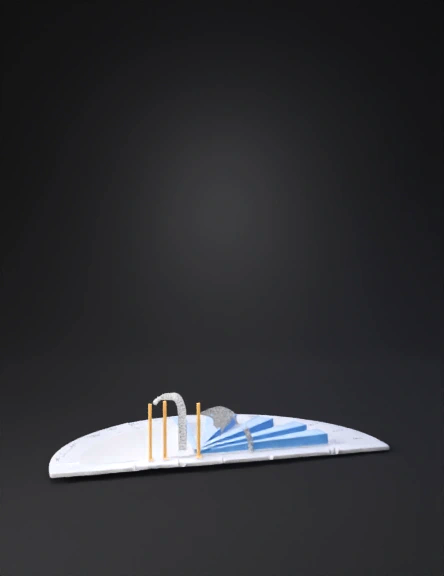
Now I will explain clearly, step-by-step, what you just saw and what you must physically make for your project. No confusion. Just structured execution. 🔵 PART 1 — YOUR MODEL BASE (Physical Structure) Step 1: Ground Construction You are given: R=40 cmR = 40 \text{ cm}R=40 cm Full Ground Area A=πR2A = \pi R^2A=πR2 A=3.1416×402A = 3.1416 \times 40^2A=3.1416×402 A=3.1416×1600A = 3.1416 \times 1600A=3.1416×1600 A=5026.55 cm2A = 5026.55 \text{ cm}^2A=5026.55 cm2 ✔ This matches the calculated result. Step 2: Divide Into 8 Equal Sectors Since: 360∘÷8=45∘360^\circ ÷ 8 = 45^\circ360∘÷8=45∘ Each sector angle = 45° Area of One Sector Asector=45360×5026.55A_{sector} = \frac{45}{360} \times 5026.55Asector=36045×5026.55 =18×5026.55= \frac{1}{8} \times 5026.55=81×5026.55 =628.32 cm2= 628.32 \text{ cm}^2=628.32 cm2 ✔ This also matches the computed value. 🔵 PART 2 — Probability Data Used We assumed this shot distribution: Sector Probability S1 0.08 S2 0.12 S3 0.18 S4 0.10 S5 0.07 S6 0.09 S7 0.14 S8 0.22 Check: Total=1.0\text{Total} = 1.0Total=1.0 ✔ Valid probability distribution. 🔵 PART 3 — Understanding the Graphs 📊 Graph 1 — Bar Chart This shows: S8 = highest (0.22) S3 = second highest (0.18) Meaning: Most runs are scored in these directions. So your model must visually show: Taller structure in S8 Slightly smaller in S3 Smallest in S5 📈 Graph 2 — Optimization Curve We sorted probabilities descending: 0.22 0.18 0.14 0.12 0.10 0.09 0.08 0.07 Cumulative: 1 fielder → 0.22 2 fielders → 0.40 3 → 0.54 4 → 0.66 5 → 0.76 So: \textbf{5 fielders give 76% coverage} This is your optimization result. 🌀 Graph 3 — Polar Plot This is the most important. It converts: Angle → θ Probability → Radius height So mathematically: x=Rcosθx = R \cos\thetax=Rcosθ y=Rsinθy = R \sin\thetay=Rsinθ z=P×kz = P \times kz=P×k Where: R = 40 cm θ = 22.5°, 67.5°, 112.5° etc (midpoints) k = scaling constant for height 🔵 PART 4 — WHAT YOU PHYSICALLY BUILD Now the actual practical model. 🔧 Materials Thermocol / MDF board (60×60 cm) Compass Protractor Colored chart paper 8 small vertical sticks (height varies) Printed probability labels Step-by-Step Construction 1️⃣ Draw Circle Radius = 40 cm Center marked 2️⃣ Mark Angles Using protractor: Mark lines at: 0° 45° 90° 135° 180° 225° 270° 315° Now you have 8 sectors. 3️⃣ Create 3D Probability Bars Height proportional to probability. Use scale: Height=Probability×30 cm\text{Height} = Probability \times 30 \text{ cm}Height=Probability×30 cm Example: S8: 0.22×30=6.6 cm0.22 \times 30 = 6.6 \text{ cm}0.22×30=6.6 cm S3: 0.18×30=5.4 cm0.18 \times 30 = 5.4 \text{ cm}0.18×30=5.4 cm S5: 0.07×30=2.1 cm0.07 \times 30 = 2.1 \text{ cm}0.07×30=2.1 cm Make 8 vertical sticks with these heights. Place each in middle of its sector. Now your ground becomes a 3D probability histogram. 4️⃣ Fielder Placement Place 5 small markers in: S8 S3 S7 S2 S4 That visually represents 76% coverage. 🔵 PART 5 — What You Say During Viva “Each vertical column represents probability density of scoring in that angular region. Optimization shows that placing 5 fielders in top probability sectors covers 76% of scoring directions.” Calm. Direct. Mathematical. 🔵 OPTIONAL — Advanced Layer (If You Want Edge) You can add a transparent sheet above the ground and draw projectile arc: y=xtanθ−gx22v2cos2θy = x\tan\theta - \frac{g x^2}{2v^2 \cos^2\theta}y=xtanθ−2v2cos2θgx2 That connects Physics + Maths. 🔵 Final Reality Check This is now: ✔ 3D ✔ Mathematical ✔ Optimized ✔ Data Driven ✔ Graph Supported ✔ Practical ✔ Unique
Detailed Info
Related Models
Enter invite code
Enter invite code to get credits!